Non-stationary RRi series
In some situations like physical exercise, the RRi series might present a non-stationary behavior. In cases like these, classical approaches are not recommended once the statistical properties of the signal vary over time.
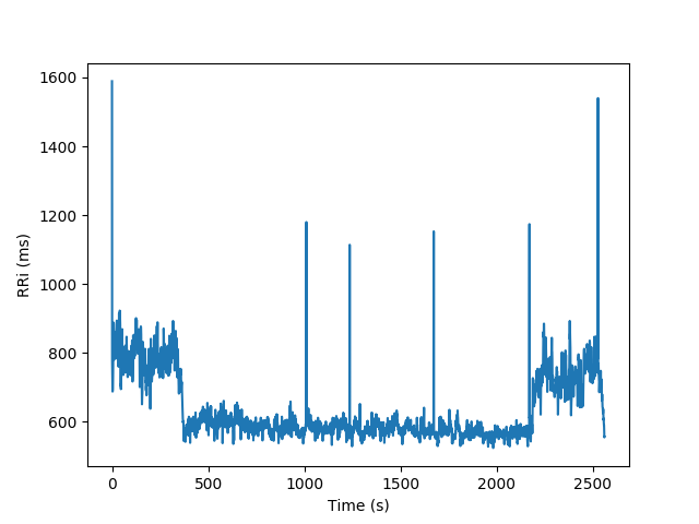
The following figure depicts the RRi series recorded on a subject riding a bicycle. Without running analysis and only visually inspecting the time series, is possible to tell that the average and the standard deviation of the RRi are not constant as a function of time.
In order to extract useful information about the dynamics of non-stationary RRi series, the following methods applies the classical metrics in shorter running adjacent segments, as illustrated in the following image:
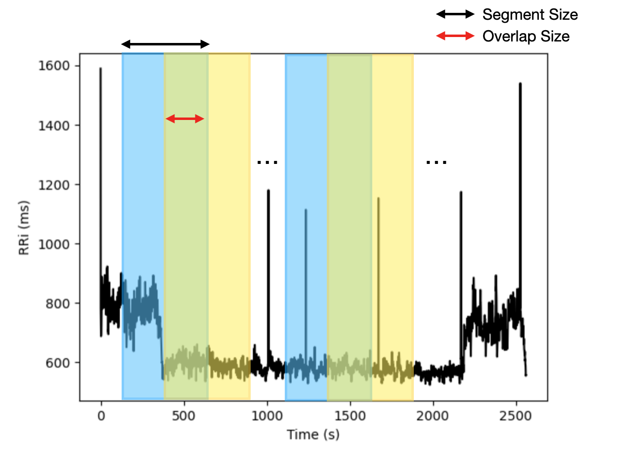
For example, for a segment size of 30s (S) and 15s (O) overlap a signal with 300s (D) will have P segments:
P = int((D - S) / (S - O)) + 1
P = int((300 - 30) / (30 - 15)) + 1 = 19 segments
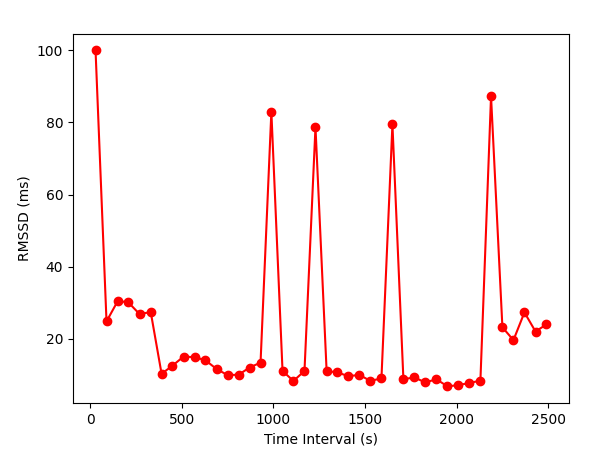
Time Varying
Time domain indices applied to shorter segments
from hrv.sampledata import load_exercise_rri
from hrv.nonstationary import time_varying

rri = load_exercise_rri()
results = time_varying(rri, seg_size=30, overlap=0)
results.plot(index="rmssd", marker="o", color="r")
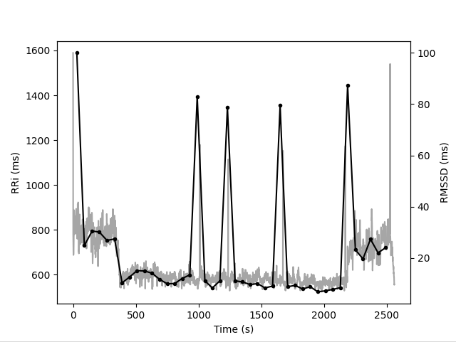
Plot the results from time varying together with its respective RRi series
from hrv.sampledata import load_exercise_rri
from hrv.nonstationary import time_varying

rri = load_exercise_rri()
results = time_varying(rri, seg_size=30, overlap=0)
results.plot_together(index="rmssd", marker="o", color="k")
Short Time Fourier Transform
To be implemented.